When you’re working on human-robot interaction research, there’s a surprisingly mundane problem that keeps showing up: the robot needs to know where things are. Specifically, in our case, the robot needed to know where small wooden magnetic blocks were sitting on a table. Not a pile of blocks. Not blocks in motion. Just blocks, on a table, waiting to be picked up.
You’d think this would be a solved problem. Point a camera at a table, detect some rectangles, done. And in a sense that’s exactly what this project does. But the gap between “detect some rectangles in an image” and “tell a robot arm exactly where to move its gripper in 3D space” turned out to be a pretty interesting engineering exercise.
This project came out of the People and Robots Lab at UW-Madison, where I was working on a collaborative robot (UR3e) manipulation pipeline. The broader goal involved task studies with magnetic blocks; before any of that could happen, the robot needed eyes. So I built it a vision system.
The Setup
The hardware side is straightforward. A USB webcam looks down at a flat table surface. Four (or more) AR tags from the Alvar library are placed on the table to define a region of interest. Wooden magnetic blocks of two sizes sit somewhere in that region. The robot arm with a Robotiq gripper waits nearby, ready to be told where to reach.
The entire system runs on ROS, with data flowing through a pipeline of specialized nodes. Camera images come in, block positions in 3D space come out. Everything in between is where the fun is.
Finding Blocks
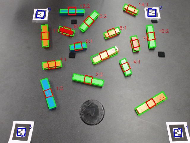
The first stage of the pipeline is pure computer vision, and I’ll be upfront about it: the algorithm is simple and somewhat brittle. It works well in controlled lab conditions, which is all we needed, but it’s not winning any robustness awards.
The detection process goes roughly like this:
- Apply Canny edge detection to find edges in the image
- Dilate and erode to strengthen the edge regions
- Convert to HSV color space and filter out anything that isn’t block-colored (this assumes the blocks sit on a dark background)
- Run another round of morphological cleanup
- Find contours in the resulting binary image
- Fit minimum-area rectangles to each contour
- Filter by area to reject noise (too small) and non-blocks (too large)
What you’re left with is a set of oriented rectangles that (hopefully) correspond to actual blocks.
Block Classification
Two sizes of blocks are used in the experiments: small and large. To tell them apart, I trained a small neural network (a single hidden layer MLP from scikit-learn) on three features extracted from each detected rectangle: the length-to-width ratio, the primary axis length in pixels, and the primary axis rotation angle.
The training data lives in a YAML file with around 40 small block samples, 60 large block samples, and a handful of counter-cases for things that aren’t blocks at all. Running `train_block_classifier.py` fits the MLP and pickles it to disk. The detection node loads the model at startup and classifies each candidate rectangle on every frame.
Is it a sophisticated deep learning pipeline? No. Does it reliably distinguish a 2:1 ratio block from a 4:1 ratio block under consistent lighting? Yes. Sometimes the right tool for the job is the boring one.
2D to 3D Problem
Here’s where things get more interesting. Knowing that a block is at pixel coordinates (320, 240) in an image doesn’t help a robot arm that thinks in meters relative to its base. You need to map from image space into world space, and for that you need some kind of calibration.
The approach I took relies on the AR tags. The Alvar library already detects AR markers and estimates their 3D poses. But I also needed their 2D image coordinates. The official `ar_track_alvar` package doesn’t publish those, so I forked it and added a second topic (`cam_pose_marker`) that outputs the 2D pixel positions of each detected tag alongside the existing 3D pose data.
With both the 2D image coordinates and the 3D world coordinates of at least four AR tags, you can compute a transformation matrix between the two spaces. The math is a pseudo-inverse computation: stack up the known 2D-to-3D correspondences, compute the least-squares optimal mapping, and apply it to any new 2D point to get its 3D position.
invX = np.linalg.pinv(X)
self._computed_position_transform = Y * invX
Two lines that do a lot of heavy lifting. The key assumption is that everything sits on a flat surface (the table), which makes the mapping well-conditioned. If blocks were floating at arbitrary heights, this approach would fall apart.
Orientation Mapping
Position is only half the story. A pick-and-place operation also needs to know how the block is rotated so the gripper can align properly. The rotation mapping works by extracting the median 2D rotation from the AR tags, finding the closest matching 3D orientation, and then applying the relative rotation to each detected block. The 3D orientation gets assembled through quaternion multiplication; the image angle gets converted to a proper rotation and composed with the table plane’s orientation from the AR data.
Getting quaternions right is one of those problems that sounds simple until you actually try it. For the calibration node (which averages multiple samples of an AR tag’s pose over time), I pulled in an implementation of Markley et al.’s quaternion averaging method. Naive component-wise averaging of quaternions produces subtly wrong results; this approach uses an eigenvalue decomposition that handles the geometry correctly. It’s based on a 2007 NASA paper, which felt appropriate for something that would otherwise silently give bad data.
Region Filtering
Not everything the detector finds inside the camera frame is a block we care about. The AR tags themselves can sometimes trigger false positives (they have strong edges and defined geometry), and anything outside the bounded region is irrelevant.
The block pose node handles this by computing the convex hull of the AR tag positions in image space (using Shapely) and rejecting any detected block whose centroid falls outside that polygon. It also applies a circular exclusion zone around each AR tag to prevent the tags from being misidentified as blocks. Simple spatial filtering, but it cleans up the output significantly.
Robot-Camera Calibration
The last piece of the puzzle is connecting the camera’s coordinate frame to the robot’s. The `robot_camera_align` node handles this through a calibration procedure: attach an AR tag to the robot’s gripper, move the arm slowly through the camera’s field of view, and let the node sample TF data over several seconds.
Position averaging is straightforward (arithmetic mean). Orientation averaging uses the same correct quaternion method mentioned earlier. The resulting transform gets saved to a YAML config file so it persists across sessions. On subsequent launches, the node just loads the saved calibration and broadcasts it to the TF tree.
The calibration procedure is manual and a bit fiddly (you need to move the arm slowly enough for good samples), but it only needs to happen once unless the camera moves.
Multi-Camera (Experimental)
I also started work on a multi-camera pipeline that would fuse data from two cameras for better coverage and accuracy. The `tf_bridge` node maps each camera’s internal TF namespace into the global tree, and a `two_camera_agreement` node matches AR markers across cameras and averages their measurements.
This part never got fully finished. It works in principle but needs more testing and refinement; it was one of those features that kept getting deprioritized in favor of actually running experiments with the single-camera setup. Sometimes shipping beats perfecting.
What Worked, What Didn’t
The single-camera pipeline worked reliably enough. Blocks got detected, classified, and located in 3D with sufficient accuracy for the robot to pick them up. The AR tag approach to 2D-to-3D mapping turned out to be robust and easy to set up; no intricate camera calibration needed beyond the basic lens parameters.
The block detection itself is the weakest link. It assumes a dark background, consistent lighting, and blocks of a specific color range. Move to a different environment and you’d need to retune the HSV thresholds (there’s a ROS service for that, at least) and possibly retrain the classifier. The algorithm is described honestly in the source code as “rather simple (and brittle).”
But that’s the nature of research infrastructure. The goal was never to build a production-grade vision system; it was to build something reliable enough that we could stop thinking about block detection and start thinking about the actual research questions. In that sense, it did exactly what it needed to do.
You can check out the source on GitHub.
Thanks for reading. Stay tuned and keep building.